In the second part of this series on pushing mesoscopic calibration to the max, Laura Oriol examines how to alter parameters for throughput at traffic signals and at major-minor priority junctions. These tips aim to show you how to avoid switching unnecessarily from meso to micro, ultimately speeding up your workflow.


Figure 1. For a free Flow speed of 100km/h – influence of Reaction time (RT) and Jam Density (JD) on flow-density diagram

The mesoscopic car-following model is a simplification of the Gipps car-following model used in microscopic simulation. If all vehicles have the same parameters, this model produces a triangular density-flow diagram (See Figure 1) that can be defined with three variables:

Free-Flow Speed

Free-flow speed is the speed that occurs when density and flow are zero. In Aimsun Next, it depends on the maximum allowed speed of the section/turn, the speed acceptance of the vehicle, and the maximum speed of the vehicle. It is represented by the positive slope of the triangular density-flow diagram.

Reaction Time

Reaction Time affects the maximum throughput and the queue propagation speed (the negative slope of the triangular density-flow diagram). In free-flow conditions and without lane-changing, the value that ensures consistency of headway, and therefore throughput, between micro and meso is RTmeso = 1.5 · RTmicro. We can observe in Figure 1 how throughput is reduced by increasing reaction times.

Jam Density

Jam Density refers to the maximum traffic density that can be observed in the section (when vehicles are stationary); it corresponds to the red dot on the diagram in Figure 1. In the car-following formula, the jam density parameter of the section is not used; what is used instead is the effective length of the vehicle, which is the sum of the length and the clearance of the vehicle, the reciprocal of which can be interpreted as a jam density.

In Aimsun Next the jam density parameter of the section is only used in queue spillback situations: to determine whether a lane is full, and to calculate how long after the first vehicle leaves a full queue another vehicle can join the back of the queue. In Figure 1 you can see how reducing the Jam Density (i.e. increasing the effective length of the vehicles) has low impact on the throughput, although it affects significantly the queue propagation speed.

Throughput at Traffic Signals

In mesoscopic simulation, vehicles are either stopped or traveling at their desired speed as there is no acceleration or deceleration in the car following model, unlike in the microscopic simulation. This simplification must be taken into account in all situations where acceleration and deceleration play an important role. It is the case at traffic signs or traffic lights, where the lack of acceleration and deceleration may yield to an overestimation of the flow unless it is compensated with the calibration of other parameters.

At signalized intersections, it is possible to use the Reaction Time at Traffic Light (RTTL) parameter to produce in meso a throughput that is more consistent with micro. This parameter is used to increase the reaction time of the first vehicle stopped at the traffic light when it switches to green. Therefore, it can be used to compensate for the lack of acceleration.

If we use the default Reaction Time at Traffic Light, 1.6s, the mesoscopic simulation is too optimistic as it achieves higher flows. Note in Figure 2, for the particular case of 1h simulation and a traffic light cycle of 60 seconds, that this difference becomes clearer the higher the speeds and the shorter the green times.

Figure 2. Micro and meso default capacity at a signalized intersection for different speeds and green times

An increase of the Reaction Time at Traffic Light in meso is sufficient to compensate the difference. The value that provides a good match mainly depends on the speed limit (Figure 3). For example, in urban areas, where traffic signals are expected and typical speeds are in the range of about 50km/h, setting a Reaction Time at Traffic Light parameter of 2.8s will compensate for the previously mentioned differences due to acceleration and deceleration.

Figure 3. Micro and meso capacity at a signalized intersection using a variable RT at traffic light in meso

Throughput at Major-Minor Priority Junctions

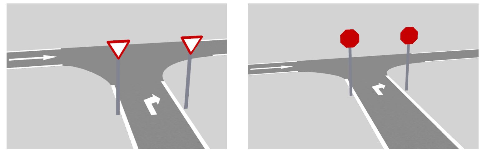
In major-minor priority junctions traffic on the minor road gives way to traffic on the major road. It is the most common form of junction control and it is normally controlled by give way or stop signs. As mentioned earlier, this is another situation that requires careful calibration in order to obtain consistent results between mesoscopic and microscopic simulation, because acceleration and deceleration play an important role. This applies to a simple T-junction controlled by a give way or a stop sign, as in Figure 4.

Figure 4. Simple T Junction

In a mesoscopic simulation the lack of acceleration and deceleration implies that give way and stop signs produce the same behaviour, while in a microscopic simulation the difference is significant. When a vehicle encounters a stop sign it stops completely before applying the gap-acceptance model, but when it encounters a give way it starts applying the model whenever the distance from the vehicle to the end of the section is less than the visibility distance. By increasing flow on the major road (conflict flow) of a simple T-junction and maintaining a constant high demand on the minor road, the results shown in Figure 5 are obtained.

Figure 5. Capacity on the minor road depending on the conflict flow on the major road with default parameters

It is clear, that in mesoscopic simulation a calibration is needed. A good start for the calibration of the mesoscopic parameters is to examine the case for zero-conflict flow, that is, no flow on the major road. It is possible to increase the Reaction Time Factor parameter on the section or to apply a lower speed on the affected turning to reduce saturation flow.

Figure 6. Capacity comparison. Calibration using Turning Speed versus using Reaction Time

Results suggest that it is better to use speed override on turning rather than reaction time factor, since we get a closer match for both flows and travel times on the minor road section (See Figure 6 and Figure 7 ). Moreover, Reaction Time Factor will apply to all turnings coming from the section, while turning speed override only affects the selected turn.

Figure 7. Travel Time comparison. Calibration using Turning Speed versus using Reaction Time