Connecting centroids to multiple sections

February 2023 — Technical note #77

Tessa Hayman

Product Specialist

Tessa Hayman explains different options for multiple centroid connections and the effects of different parameters and assignment algorithms.

A common question in transport modeling training courses is, “Should I connect my centroids to multiple sections and what happens if I do?”

In this technical note we will look at centroid connections, the different options for them, and what goes on in the background for each type of network loading within an Aimsun Next model.

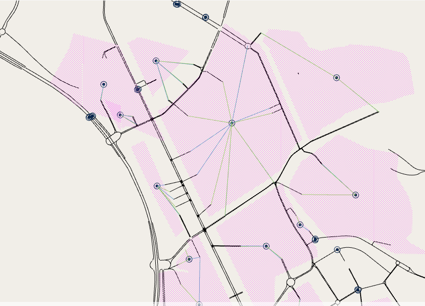
Using only one entrance connection and one exit connection for each centroid is the most convenient option, as this makes it easier to keep track of the flow changes caused by matrix adjustments, making validation and calibration easier. However, multiple connections may be required when the zone is large and therefore has multiple accesses/egresses, or to maintain consistency with a planning model that provides the demand.

When a centroid has multiple connections, the traffic must choose a connection, and this can happen as part of the path choice or as a separate calculation, depending on the assignment algorithm and on the settings defined for the centroid. This technical note will explain the effects of the different parameters and algorithms.

Dynamic assignments

For dynamic experiments (macro-meso, meso-micro, meso and micro) connections have no cost, but there are several parameters that control how each vehicle chooses between multiple entrance and exit connections and how the paths between them are calculated and evaluated
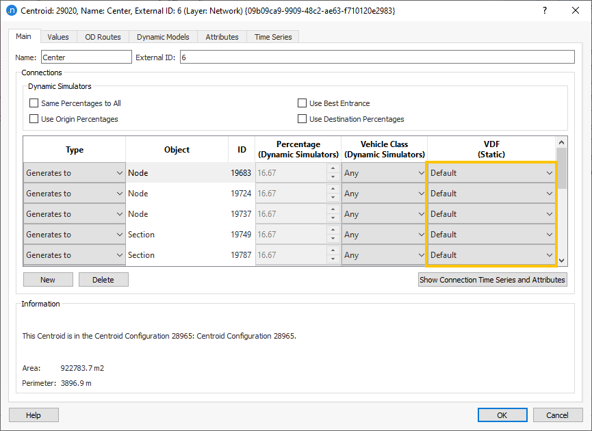
These are defined in the centroid properties:
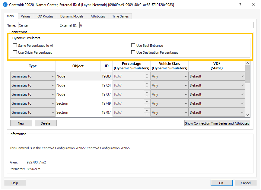
If no box is ticked, then the vehicles choose a connection according to the cost to their destination, as calculated using the initial and dynamic cost functions. In general, this means that vehicles use the entrance(s) that will get them to their destination quickest, and therefore this should be the default and preferred setting.

 
For dynamic user equilibrium (DUE), when using Dijkstra, at the end of each departure interval and each iteration, a new path tree is calculated but only one path, the one with the least cost, is added to the path list, even if the origin centroid has multiple connections. When using A-star just one point-to-point path is calculated. The path is added to the path set up to the maximum number of paths set in the dynamic traffic assignment tab, and the vehicles are distributed between them according to the proportions calculated by the MSA, WMSA or gradient-based algorithm.
 
Therefore, if split percentages are not manually set, the assignment ultimately determines the split of the trips between the different entrance and exit connections: in the case of SRC, the discrete choice model applied to the cost of the different options; in the case of DUE, the MSA, WMSA or gradient-based algorithm.
 
On the other end, if you set entrance or exit connection percentages (or both) each connection is considered as a separate origin or/and destination both in the path calculation and evaluation, and in the computation of convergence measures.
 
If you use destination percentages, you are first splitting the demand between the exit connections with the given proportions, then the path calculation will assign the vehicles from their origin to their respective destination connection. Therefore, if you use destination percentages, you are forcing the path finding process to calculate one path tree for each exit connection, which increases the runtime and memory consumption as if you had as many destination centroids as exit connections.
 
If you use origin percentages, you are first splitting the demand between the entrance connections with the given proportions, then the path calculation will assign the vehicles from their respective origin connection to their destination.
 
Same percentages to all has the same effect as using both origin and destination percentages, while setting for each a value equal to 100% divided by the number of entrance and exit connections respectively.
 
When you use percentages, the max number of paths is applied to each origin connection-destination centroid (if using only origin percentages), to each origin centroid-destination connection (if using only destination percentages) or to each origin connection-destination connection (if using both); therefore, the max number of paths between an OD pair becomes the total combination of possible entrance/exits multiplied by the max number of paths parameter.
 
Note that the percentages you set are applied homogenously to all vehicles that have that origin (regardless of their destination – provided there is feasible path) or destination (regardless of the origin – provided there is a feasible path) and therefore vehicles may be assigned to an entrance or exit that doesn’t allow them to get quicker to their destination.
 
For this reason, you should not use percentages just as a way to spread traffic, or to obtain an observed count on the entrances/exits; they should only be used in specific situations, generally when the reason to pick one or another connection is not related to the convenience of the path, i.e. when you want to obtain the same result of splitting a centroid into multiple centroids (as with the split/join feature included in Aimsun Next 22), but without modifying the network. It is advised that if you have known percentage splits, that you split your centroids as it can be beneficial when calibrating and validating the model, particularly in adjustment.
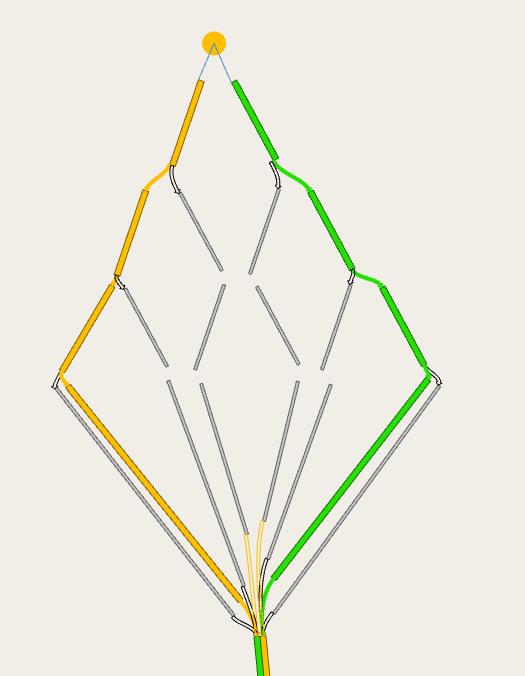
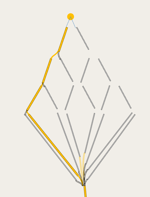
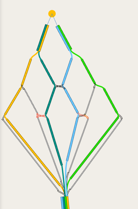
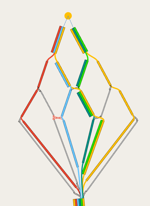
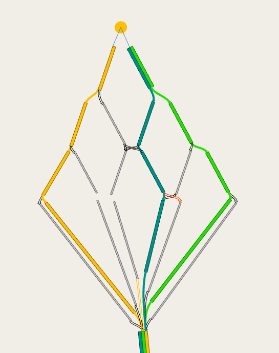
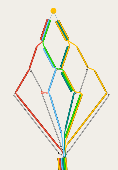
Example showing the differences between stochastic route choice (with default settings and with use best entrance) and dynamic user equilibrium when max number of paths is set to 3 and Dijkstra shortest path algorithm is used.
Model SRC with default options SRC with Use Best Entrance DUE
Step Path list Description Path list Description Path list Description
1 Image In the first interval of the warm or main simulation, calculate using the ICF the least cost path tree. When there are multiple entrance connections, the tree will provide one path per entrance connection for the same OD. Add all these to the path set. With two entrance connections, it can contain up to two paths. If there are already multiple paths, calculate the probability of choice by applying the discrete choice function. Image In the first interval of the warm or main simulation, calculate using the ICF the least cost path tree. Add only the least cost path to the set for all intervals. There is one path in the path set. Assign all vehicles to that path. Image In the first iteration calculate, using the ICF the least cost path tree. Add only the least cost path to the set for all intervals. There is one path in the path set. Assign all vehicles to that path. Note that the path is the same for all intervals.
2 Image In the next cost interval, using the DCF and the costs at the end of the previous interval, calculate the least cost path tree. When there are multiple entrance connections, the tree will provide multiple paths for the same OD. Add all these to the path set. With two entrance connections, it can contain up to four paths. Select from the path set the 3 paths with lower cost and calculate the probability of choice by applying the discrete choice function. Image In the next cost interval, using the DCF and the costs at the end of the previous interval, calculate the least cost path tree. Add only the least cost path to the set. There are now (up to) two paths in the path set. Calculate the probability of choice by applying the discrete choice function. Image In the next iteration, for each interval, calculate, using the DCF and the costs at the end of the same interval in the previous iteration, the least cost path tree. Add only the least cost path to the set.There are now (up to) two paths in the path set. Split vehicles equally.
3 Image In the next cost interval, using the DCF and the costs at the end of the previous interval, calculate the least cost path tree. When there are multiple entrance connections, the tree will provide multiple paths for the same OD. Add all these to the path set. With two entrance connections, it can contain up to six paths. Select from the path set the 3 paths with lower cost and calculate the probability of choice by applying the discrete choice function. Image In the next cost interval, using the DCF and the costs at the end of the previous interval, calculate the least cost path tree. Add only the least cost path to the set. There are now (up to) three paths in the path set. Calculate the probability of choice by applying the discrete choice function. Image In the next iteration, for each interval, calculate, using the DCF and the costs at the end of the same interval in the previous iteration, the least cost path tree. Add only the least cost path to the set.There are now (up to) three paths in the path set. Split vehicles equally.
4 Image In the next cost interval, using the DCF and the costs at the end of the previous interval, calculate the least cost path tree. When there are multiple entrance connections, the tree will provide multiple paths for the same OD. Add all these to the path set. With two entrance connections, it can contain up to eight paths. As the two new paths from the path tree already exist in the path set, only 6 paths are in the path set. Select from the path set the 3 paths with lower cost and calculate the probability of choice by applying the discrete choice function. Image In the next cost interval, using the DCF and the costs at the end of the previous interval, calculate the least cost path tree. There are now (up to) four paths in the path set. Select from the path set the 3 paths with lower cost and calculate the probability of choice by applying the discrete choice function. Image In the next iteration, since we have reached the max number of paths, no new path trees are calculated. The cost of the paths in the set is recalculated, using the DCF and the costs at the end of the same interval in the previous iteration. The vehicles are split according to the MSA, WMSA or gradient-based algorithm.

How are the trips assigned to each path type in a one-shot?

    1. On vehicle generation, each vehicle is given a random number by the random seed.
    2. The random number is used to select its path source. It will decide if it is going to use a user defined OD route (if available), a path from the input path assignment file (if available), or the stochastic route choice method for the experiment. This is based on the percentage of vehicles that are using each source.
    3. If the vehicle is going to use a route from the input path assignment file, the path is chosen according to the probability of each path from the path assignment file. This implies that if the path assignment file was generated using connector percentages or “use best entrance” the effect of those parameters will influence the vehicles that use a route from the input path assignment file.
    4. If the vehicle is going to use stochastic route choice, the path is chosen according to the probability of the path given by the connector settings and the route choice algorithm.
      1. If user defined origin or/and destination percentages (or equal percentages), then each entrance or/and exit is considered as a different centroid and the paths are selected using the route choice algorithm from each entrance/exit pair
      2. If no percentages are set or “use best entrance”, the path set is created, and the path is chosen according to the rules described in the table above for stochastic route choice.

Static Assignments

In static assignments the choice of the entrance and exit connections is solely controlled by the path calculation, which is influenced by the VDF set for the connection. If this is not defined, this will use the default VDF as the cost which is travel time in minutes. This uses the section speed of the entrance section and the distance of the connector to give a free flow travel time. If you are using a generalized cost in the rest of your model, then the VDF of the centroid connection will need to be altered so that it is consistent. This can be changed in the centroid menu.

Note that as a hybrid macro-meso is a dynamic assignment, the choice of the connections is controlled as described in the previous chapter.


What happens when you use the path assignment from a previous run?

This depends on the type of experiment that the path assignment file is from and the type of experiment it is being used for.

  • Static assignment with static path assignment input: the percentage split between the paths and thus the connectors is given by the percentage assigned to each path in the path assignment file for the first iteration. Subsequent iterations will alter the percentages and the path set according to the static assignment algorithm.
  • Static assignment with dynamic path assignment input: you cannot run a static assignment with a dynamic path assignment file.
  • SRC dynamic assignment with static path assignment input: the vehicles that are using “path assignment” as their source of paths will follow the paths and probabilities of choice in the path file, which means that the percentages in the connections or use best entrance have no effect on them (they have only effect on vehicles following a path provided by the stochastic route choice). Note that if there was no trip between the OD pair in the run that generated the path file, the vehicle will use stochastic route choice.
  • SRC dynamic assignment with dynamic path assignment input: the vehicles that are using “path assignment” as their source of paths will follow the paths and probabilities of choice in the path file, which means that they will be affected by the percentages in the connections or use best entrance set when the path file was generated (the ones currently set have only effect on vehicles following a path provided by the stochastic route choice). Note that if there was no trip between that OD pair in the run that generated the path file, the vehicle will use stochastic route choice (so be sure to set the same random seed).
  • Dynamic user equilibrium with static or dynamic path assignment input: vehicles are first split according to the origin or/and destination percentages currently set (if any), then the initial path set and probabilities of choice are read from the path file (with some modifications in case of inconsistent settings: if it comes from a static assignment, or from a dynamic assignment with no connection percentages, and the connections currently have percentages, the probabilities of choice are rebalanced to 100% per connector; if it comes from a dynamic assignment with connection percentages, and the connections currently don’t have percentages, the first x paths for each OD are taken and their probabilities rebalanced to 100%).


Geometry configurations:

If a centroid is connected to one or more sections which are not present in the current active view, then the percentage split might not add up to 100% for each combination of Geometry Configurations. There are several options to cope with this situation:

  1. Allow Aimsun Next to set the percentage split for all sections by either setting the connectors to default, same percentages to all or use best entrance.
  2. If a centroid is connected to sections 1,2,3 in one configuration and 1,2,4 in another, ensure the splits for 3 and 4 are the same.
  3. Edit the connecting sections to ensure there is a single common section connecting to the centroid for all Geometry Configurations.
  4. Split the centroid into one centroid per connection using the split centroid tool and change the connections in the geometry configuration.
  5. Duplicate the centroid and edit the demand and the splits in different matrices for each copy of the centroid. Create new Traffic Demands to hold the edited matrices and select a Traffic Demand for the scenario that is consistent with the Geometry Configuration.

More technical notes

C/ACC controller in Aimsun Next

October 2021: In this article, Martin Hartmann explains and demonstrates Aimsun Next microsimulation of vehicles equipped with cooperative adaptive cruise control (CACC).

Aimsun
  • Got a question? Get in touch.

    We are here to help!

SHARE

Cite Aimsun Next

Aimsun Next 24

Aimsun (2024). Aimsun Next 24 User’s Manual, Aimsun Next Version 24.0.0, Barcelona, Spain. Accessed on: April. 16, 2024. [Online].

Available: https://docs.aimsun.com/next/24.0.0/

Aimsun Next 24

@manual {AimsunManual,
title = {Aimsun Next 24 User’s Manual},
author = {Aimsun},
edition = {Aimsun Next 24.0.0},
address = {Barcelona, Spain},
year = {2024. [Online]},
month = {Accessed on: Month, Day, Year},
url = {https://docs.aimsun.com/next/24.0.0},
}​​​​​​​​​​​​​​​

Aimsun Next 24

TY – COMP
T1 – Aimsun Next 24 User’s Manual
A1 – Aimsun
ET – Aimsun Next Version 24.0.0
Y1 – 2024
Y2 – Accessed on: Month, Day, Year
CY – Barcelona, Spain
PB – Aimsun
UR – [In software]. Available:
https://docs.aimsun.com/next/24.0.0/