
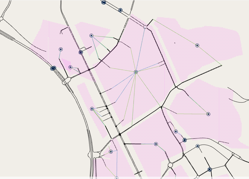
Walk or take the bus? Modeling mode choice with dynamic transit assignment.
Dynamic Transit Assignment in Aimsun Next for pedestrians to walk or to walk and take transit to reach their destination.


Dynamic assignments
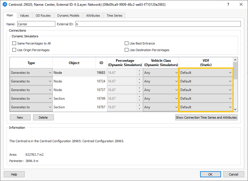
For dynamic experiments (macro-meso, meso-micro, meso and micro) connections have no cost, but there are several parameters that control how each vehicle chooses between multiple entrance and exit connections and how the paths between them are calculated and evaluated
These are defined in the centroid properties:
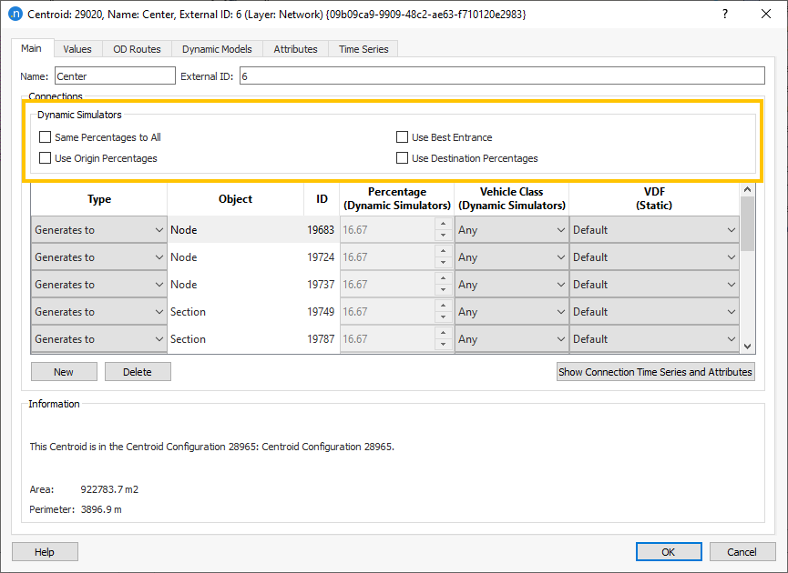
If no box is ticked, then the vehicles choose a connection according to the cost to their destination, as calculated using the initial and dynamic cost functions. In general, this means that vehicles use the entrance(s) that will get them to their destination quickest, and therefore this should be the default and preferred setting.
| Model | SRC with default options | SRC with Use Best Entrance | DUE | |||
|---|---|---|---|---|---|---|
| Step | Path list | Description | Path list | Description | Path list | Description |
| 1 | 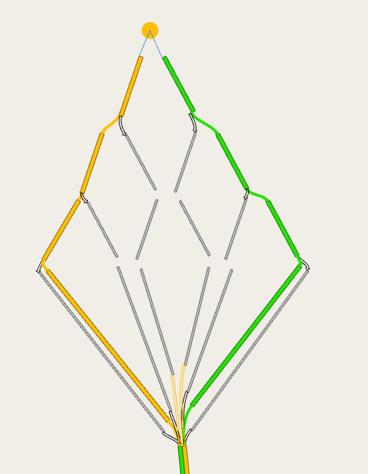 |
In the first interval of the warm or main simulation, calculate using the ICF the least cost path tree. When there are multiple entrance connections, the tree will provide one path per entrance connection for the same OD. Add all these to the path set. With two entrance connections, it can contain up to two paths. If there are already multiple paths, calculate the probability of choice by applying the discrete choice function. | 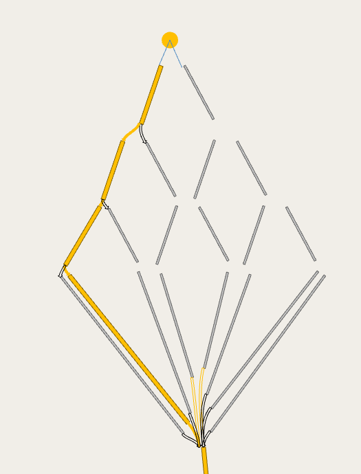 |
In the first interval of the warm or main simulation, calculate using the ICF the least cost path tree. Add only the least cost path to the set for all intervals. There is one path in the path set. Assign all vehicles to that path. | |
In the first iteration calculate, using the ICF the least cost path tree. Add only the least cost path to the set for all intervals. There is one path in the path set. Assign all vehicles to that path. Note that the path is the same for all intervals. |
| 2 | 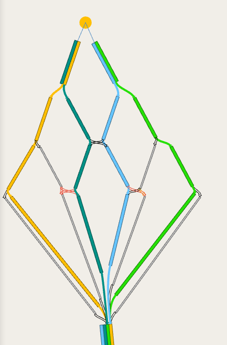 |
In the next cost interval, using the DCF and the costs at the end of the previous interval, calculate the least cost path tree. When there are multiple entrance connections, the tree will provide multiple paths for the same OD. Add all these to the path set. With two entrance connections, it can contain up to four paths. Select from the path set the 3 paths with lower cost and calculate the probability of choice by applying the discrete choice function. | |
In the next cost interval, using the DCF and the costs at the end of the previous interval, calculate the least cost path tree. Add only the least cost path to the set. There are now (up to) two paths in the path set. Calculate the probability of choice by applying the discrete choice function. | |
In the next iteration, for each interval, calculate, using the DCF and the costs at the end of the same interval in the previous iteration, the least cost path tree. Add only the least cost path to the set.There are now (up to) two paths in the path set. Split vehicles equally. |
| 3 | 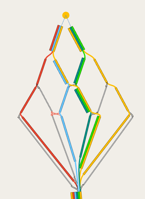 |
In the next cost interval, using the DCF and the costs at the end of the previous interval, calculate the least cost path tree. When there are multiple entrance connections, the tree will provide multiple paths for the same OD. Add all these to the path set. With two entrance connections, it can contain up to six paths. Select from the path set the 3 paths with lower cost and calculate the probability of choice by applying the discrete choice function. | 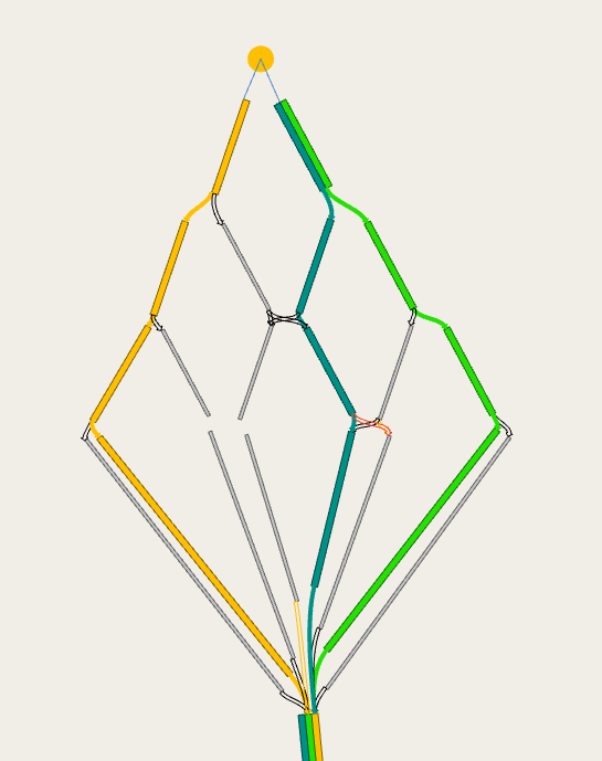 |
In the next cost interval, using the DCF and the costs at the end of the previous interval, calculate the least cost path tree. Add only the least cost path to the set. There are now (up to) three paths in the path set. Calculate the probability of choice by applying the discrete choice function. | |
In the next iteration, for each interval, calculate, using the DCF and the costs at the end of the same interval in the previous iteration, the least cost path tree. Add only the least cost path to the set.There are now (up to) three paths in the path set. Split vehicles equally. |
| 4 | 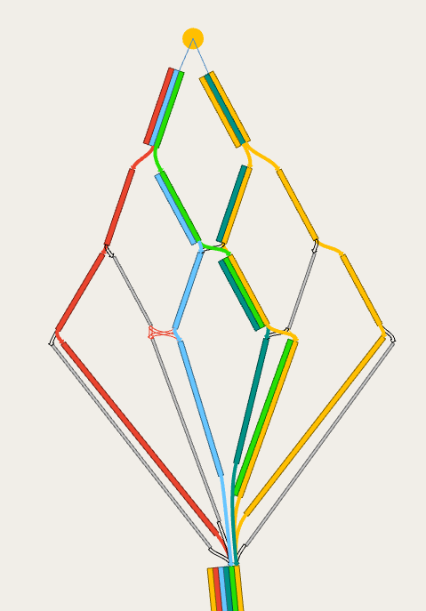 |
In the next cost interval, using the DCF and the costs at the end of the previous interval, calculate the least cost path tree. When there are multiple entrance connections, the tree will provide multiple paths for the same OD. Add all these to the path set. With two entrance connections, it can contain up to eight paths. As the two new paths from the path tree already exist in the path set, only 6 paths are in the path set. Select from the path set the 3 paths with lower cost and calculate the probability of choice by applying the discrete choice function. | |
In the next cost interval, using the DCF and the costs at the end of the previous interval, calculate the least cost path tree. There are now (up to) four paths in the path set. Select from the path set the 3 paths with lower cost and calculate the probability of choice by applying the discrete choice function. | |
In the next iteration, since we have reached the max number of paths, no new path trees are calculated. The cost of the paths in the set is recalculated, using the DCF and the costs at the end of the same interval in the previous iteration. The vehicles are split according to the MSA, WMSA or gradient-based algorithm. |
Static Assignments
In static assignments the choice of the entrance and exit connections is solely controlled by the path calculation, which is influenced by the VDF set for the connection. If this is not defined, this will use the default VDF as the cost which is travel time in minutes. This uses the section speed of the entrance section and the distance of the connector to give a free flow travel time. If you are using a generalized cost in the rest of your model, then the VDF of the centroid connection will need to be altered so that it is consistent. This can be changed in the centroid menu.
Note that as a hybrid macro-meso is a dynamic assignment, the choice of the connections is controlled as described in the previous chapter.
What happens when you use the path assignment from a previous run?
This depends on the type of experiment that the path assignment file is from and the type of experiment it is being used for.
Geometry configurations:
If a centroid is connected to one or more sections which are not present in the current active view, then the percentage split might not add up to 100% for each combination of Geometry Configurations. There are several options to cope with this situation:
Dynamic Transit Assignment in Aimsun Next for pedestrians to walk or to walk and take transit to reach their destination.

本技术注解将解释Aimsun Next中微观和中观仿真中不同的随机性来源以及如何控制它们。
