
Automatic model file management
Dimitris Triantafyllos explains how to use the Aimsun Next project folder structure to automatically manage model files.


The Real Data Set module in Aimsun Next accepts most of the known data types used for a simulation model. An RDS reader module can be easily configured to retrieve data from text-based files or positional data held in a GPS-based standard format. More details on the RDS reader can be found in the User Manual.
Sometimes RDS can contain a large amount of data. To save retrieve/analysis time it can be filtered by subnetwork or by time. For example, in a test model, two sources of data were used: motorway data and signalized intersection data. They are combined in the RDS as shown in Figure 1. The original data set was recorded for 24 hours at 15min intervals. When analyzing a particular model period such as the afternoon peak, we do not need to use the whole data set. A time filter can be applied to retrieve information from the required time interval (e.g. 2 to 7 pm). An example of the retrieved data for the whole day vs PM peak is shown in Figure 2.
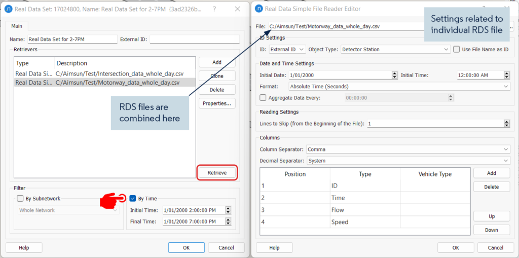
Figure 1: An example of the RDS input window
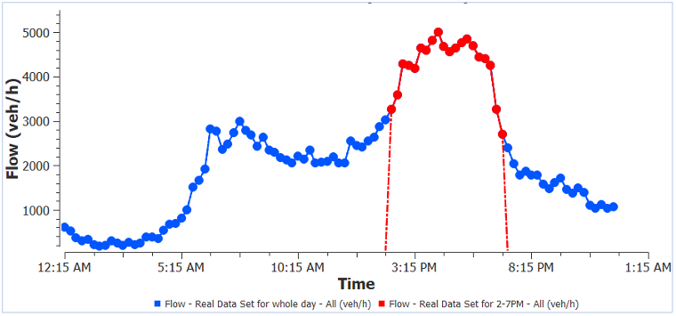
Figure 2: An example of detector flow with whole day vs PM peak data
During the data retrieval process, a set of standard checks are performed. These include invalid Date/Time, initial time and interval, invalid or missing data values, negative and NaN data values, missing objects in the model as per the RDS ID setting, and IDs with multiple objects in the model. Also values for time, object, and vehicle type are checked in every scanned record. Any anomalies found in the data are reported in the result tab and a success/fail message of the retrieving process is printed in the Log window for every file scanned. An example of the retrieved result for the test RDS reported before is shown in Figure 3 below.
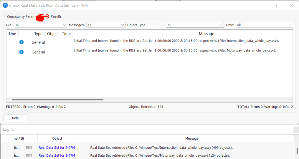
Figure 3: RDS retrieve results tab (top) and Log window (bottom)
The Real Data Consistency Checker ensures data is consistent with the flow, speed, and occupancy values. The default outlook of the consistency checker is shown in Figure 4. Please note that the default values are a guide only. More discussion on the choice of parameter values can be found later.
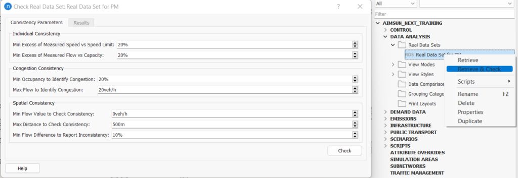
Figure 4: RDS consistency checker with default values
Min Excess of Measured Speed vs Speed Limit: Identifies any individual data point where the RDS speed value is 20% higher than the section (or turn) speed limit coded in the model. Driver behavior, location of the study area, and time of analysis (peak, off-peak) can influence this selection. A quick summary of the data can provide better insight into this threshold value. The focus should be given to identifying outliers, and data entry errors. For example, in a road section with speed limit of 100km/hr, a speed entry of 300 km/hr is a data entry error while 150 km/hr can be an outlier or not.
Min Excess of Measured Flow vs Capacity: Identifies any individual data point where the RDS flow value is 20% higher than the section (or turn) capacity coded in the model. If the data are retrieved by lane (e.g. lane detector) they will be compared with lane capacity.
Congestion consistency: A data point is identified as congested when its occupancy is high and its flow is low; Min Occupancy to Identify Congestion and Max Flow to Identify Congestion define the thresholds for high occupancy and low flow. Please note that in the case of multilane objects (section or detector station) the default aggregation process uses flow value as the sum of available lane flows while the occupancy is averaged over available lane occupancies. Therefore, you will have to select a higher value of Max Flow to Identify Congestion when you have detectors covering multiple lanes.
Spatial consistency: It can identify inconsistency of flow (or count) between two measured points within a specified distance. It can also identify inconsistencies between incoming and outgoing flow in a node. The algorithm requires three parameters:
Notes on spatial consistency check
When the record corresponds to a partial value (not covering all the lanes of the section) data on the missing lanes will be looked for within 50m. When not found, this record will not be checked for spatial consistency.
The possible difference in flow due to distance between the measurement points is taken into account by calculating an approximate storage capacity if all vehicles were stopped between these two points. When there are no geometry interferences between two points (i.e., no merge/diverge or centroid connections) but the flow difference minus storage capacity between both points exceeds the Min Flow Difference to Report Inconsistency an error will be issued, because one of the observations should be theoretically incorrect.
For individual and congestion consistency check, the RDS consistency check looks at each observation at each time point and applies the algorithm. For spatial consistency check, it looks at multiple objects within each time period. When the dataset is stored at small time intervals (e.g.,15min) it could generate a big list of warnings which could be overwhelming and sometimes difficult to manage. For example, in the test model mentioned before, the dataset was 24 hours in duration with 15min intervals. To reduce runtime the dataset can be trimmed to 5hrs (2-7 pm), which is the analysis period, using the filter options described above. The consistency check with the default value generated 849 messages in total. The filter option would help to separate the output by message types, object type (e.g. section, node, detectors), and by RDS file.
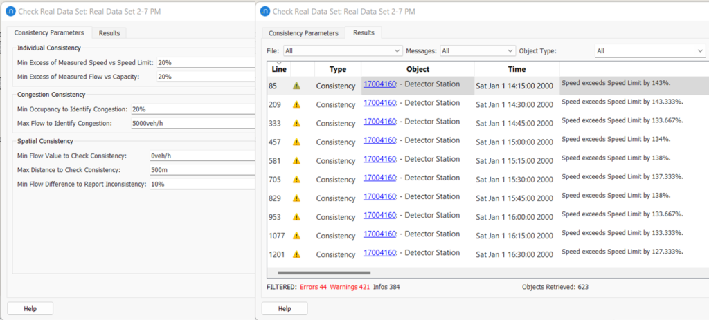 Figure 5: Example of RDS consistency check messages
If we look closely at Figure 5, for the same detector station same error message is generated for each time point. Depending on the application of the data we may need to look at each time interval and sometimes aggregated data over a period would be appropriate. In the following sections, some common applications of this tool are discussed.
The static OD adjustment process looks at the simulated volume and compares that with the RDS volume. The data does not need to be time dependent. We are mostly interested in flow inconsistency as it could negatively impact the adjustment process. We can aggregate data by the simulation period. For example, in the test model, we have utilized the automatic aggregation option available in the RDS reader as shown in Figure 6.
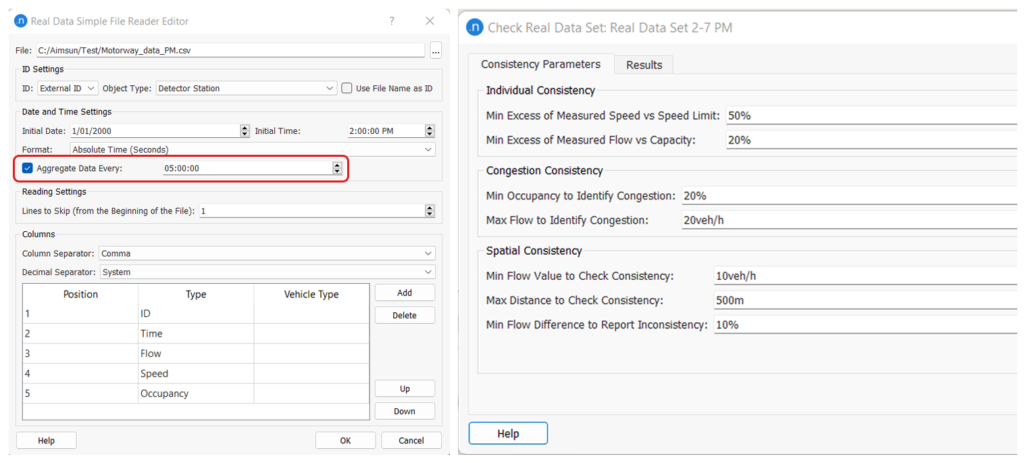
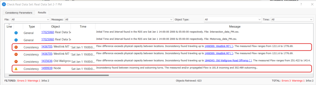
Figure 6: RDS consistency check with aggregated data
When the consistency check is performed on the aggregated data, the number of spatial consistency errors has dropped from 44 to 3. When we are not interested in speed values, a high threshold for Measured Speed vs Speed Limit can be used to avoid reports on speed errors. Similarly, the occupancy checks can also be avoided with a low value for Max Flow to Identify Congestion.
If we look at the description of the first error, it says that the two section detectors have a flow difference of 565 (1776-1211) vehicles. As there are no other geometry interferences one of the flow values must be incorrect. In this case, the lower flow value was caused by a faulty detector. In the last warning message, the calculation for the node is based on incoming and outgoing flow as shown in Figure 7. Interestingly, data for one outflow turn was missing which was recalculated by the downstream node information.
Manually identifying such inconsistency within the data would take a long time. Whereas the RDS consistency check is mostly automatic and runs within seconds to provide useful information about flow variation. We should update/avoid the inconsistent detector for the Static OD adjustment process.
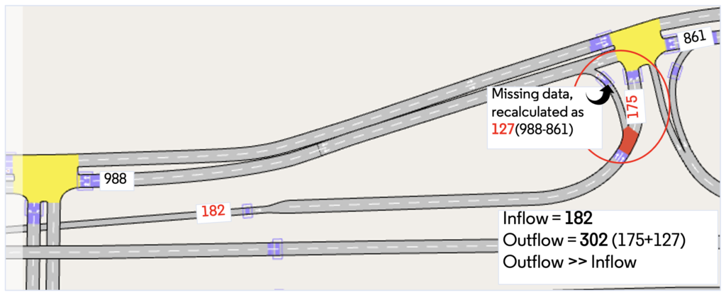
Figure 7: Calculation of flow for node inconsistency check (the numbers denote average flow)
Speed data are important for model calibration and validation. The process identifies speed anomalies by comparing them with the section (or turn) speed limit. Speed data is time-dependent and should be analyzed by each time point or can be aggregated by the model reporting time interval. Sometimes this analysis can also help us to identify anomalies in section speed limit. For example, if the speed limit data for the model is outdated, the latest RDS can identify possible locations where changes are required. In this test model, warnings for the ramp speed are frequently reported. One example is shown in Figure 8 where the ramp speed limit was set to 60 km/hr and the motorway speed limit was 110 km/hr. The ramp speed at the detected location may not be justified as the driver would have just started to slow down after exiting the motorway. The ramp speed may be updated based on the RDS speed value.
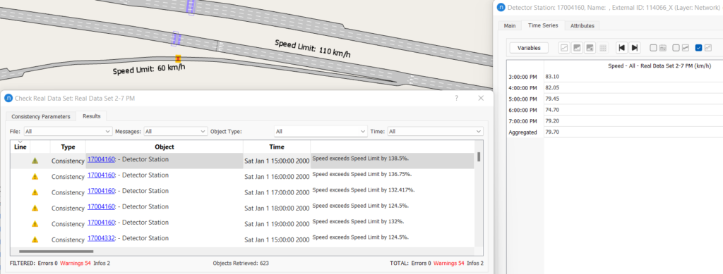
Figure 8: Identifying section speed limit anomalies from RDS
With flow and occupancy data, the congested locations can be identified from the RDS. This result is marked as information. The identified locations can be used to create congested section grouping to assist the Static OD adjustment process. It will also help the model validation process as it informs typical real-life locations where the congestion occurred. In the test model, we have used 1-hour aggregation to report congestion consistency. The parameter choice should be based on the flow and occupancy value observed in some typical congested locations. In Figure 9 the flow and occupancy profile of two typical congested locations (AM and PM) on the motorway is shown. Based on this profile, the parameter value for Max Flow to Identify Congestion is set to 4200 vehicles per hour and Min Occupancy to Identify Congestion is set to 25%. A lower value for min occupancy could produce a lot of cases with mild congestion or sections at capacity. An example of the Congestion consistency outputs is shown in Figure 9 with parameter values used. It identifies, for example, that the detector 4421 was partially congested during the PM period.
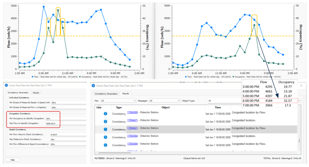
Figure 9: An example of congestion consistency setup and results
Dimitris Triantafyllos explains how to use the Aimsun Next project folder structure to automatically manage model files.

Mohammad Saifuzzaman shows how the Aimsun Real Data Set Checker makes it quicker and easier to create clean datasets and examines some different use cases.
