How to use random forests to predict mobility patterns

Ferran Torrent
Senior Data Scientist at Aimsun
In the previous article, we extracted a set of nine flow patterns from a two-year dataset (2018-2019). We extracted patterns using clustering and they were distributed as shown in the illustration below. However, now there is no direct mapping between the day of the week and patterns. The rules for assigning a pattern to each day are more complicated Obviously, if we have the measured flow of each day, we can just calculate the distance between each day and each pattern and there we have it. However, the true value lies in doing it in advance, without the measured flow. We can use all the work that we saved in using clustering to extract patterns when we need to predict how to assign a pattern.

Fortunately, we have ‘supervised learning’ to help us train our model to predict the right pattern. We simply need to decide which candidate features (or explanatory variables) may be useful for the prediction task and candidate type of models to build, but after this step, it’s just a matter of comparing results and iterating.
The need to predict traffic patterns without using the flow of such a day applies to forecasting for the next day or even several days ahead. If we cannot rely on traffic measurements, we can use calendar features such as holidays, days of the week, or season. Other features, such as weather or special events, could also be useful if their forecasts are available. For example, we may know if there will be an important football match in the stadium in the middle of the city, but we will not know if there will be an accident that blocks several lanes of one of the main roads.
Regarding the type of model, it can be any that is suitable for a multiclass classification. For example, we can test logistic regression, or decision trees, or neural networks. In this example we’ll test logistic regression and random forests.
Logistic regression
Logistic regression learns a linear combination of the explanatory variables that are then input to a sigmoid function to output the probability of an example of being negative or positive. The weights of the linear combination are the parameters learned by minimizing cross-entropy. Basically, the model learns to output the highest possible probability when the class is 1 and the lowest possible probability when the class is zero. With this procedure the model learns the best hyper-plane that divides positive and negative examples. In our case we have 9 patterns, so we use a logistic regression that instead of using a sigmoid function uses a softmax. Softmax is a generalization of sigmoid function so that instead of giving a single number (probability of class 1), it returns N numbers, where N is the number of classes and so each number represents the probability of each class. With this, the model learns to output high probability for the right class and low probability for the others.
Random forests
Random forests are ensembles of decision trees. Decision trees do not split the space with linear hyper-planes, they split them with questions such as, Is X greater than A, where X is a particular explanatory variable and A is a particular value that X can take? Therefore, a tree represents a set of rules that define a region. Trees are built so that each region that is defined by the leaves of the trees only contains examples of the same class, which maximizes the purity of each region. There are different metrics such as scikit-learn implementation, which lets you choose between the Gini Index or entropy. In this case, we’ll use entropy as it usually performs better with unbalanced datasets, like the one we have. On the other hand, entropy is more expensive to compute than the Gini Index.
If decision trees already split the solution space, why do we need an ensemble? The main problem is that when building decision trees there is a lot of freedom. So, to be efficient there are a set of heuristics used to choose such as the decision variable, the splitting point… These heuristics do not guarantee the optimal solution. To solve this problem, we can build many decision trees and average their predictions. Another problem related to the flexibility of decision trees is overfitting. It means that we can build a decision tree that very accurately divides the solution space, but that such division does not generalize well to unseen data. To regularize the flexibility of the decision trees we can limit the number of splitting points or the number of variables to use. However, doing this we may end up with a limited tree that does not split the space accurately. On the other hand, by building many decision trees and averaging their predictions we can have many bad trees (or weak learners) that in combination are a good model. To put it simple, random forests reduce the variance (this means that increase how de model generalizes) at the cost of building more trees. Nevertheless, considering the speed at which a tree is built, we can say that random forests reduce the variance with respect to decision trees at no cost.
Cross-validation
Machine learning algorithms enjoy great flexibility when they are built, but this flexibility is a double-edged sword: it lets us build models that can emulate any kind of function, but we can end up with a model that emulates a function that is not related to the true function and so it will perform poorly with new unseen data. When the latter occurs, we say the model is overfitted to the training data. To avoid this there are the regularization techniques that limit the freedom of the models when they are built. But to see if the model generalizes it is necessary to test it with data not seen in the training period. In the big data era with hundreds of thousands (or even millions) of examples, it is only necessary to split the dataset into a training set and a test set (for example 90% and 10%). But this is not the case faced here. We have 730 days (about 2 years); if we keep 73 days for testing, the way we choose these days will have a significant impact on performance. For example, if the 73 days are only Monday-Friday with no holidays we won’t see how the model behaves on atypical days such as Christmas. On the other hand, if the 73 days fall mostly in January and December, we won’t get a global picture of how well the model behaves for “normal” weeks. A good option then, is to do k-fold cross-validation. This means dividing the dataset between train and test but do this k times. So, each time we will have a different train and test sets and we will build and test a model with them. At the end, we can merge the results and see how well the models perform on the whole dataset, but without seeing the predicted examples in the training process. This will give insight into how well a model will generalize to new unseen data.
This way of validating the models is sometimes perceived as unnecessary in the transport industry, probably due to its history of modelling traffic for planning purposes with very scarce data. Obviously cross validation is not useful if the data consists of 1 day of flow data at two points of a network and the objective is long-term planning for years into the future. But when the objective is to perform real-time forecasting for the next minutes, hours or days and we have a dataset of months of data from hundreds of points in the network, then it is necessary to validate the model with unseen data before deploying it. At @aimsun we take this very seriously and we never deploy a model with significant differences in the accuracy using the training set or test set that hints at possible overfitting.
Results
I use 5-fold cross-validation to train and test logistic regression models and random forests with 1000 trees with a maximum depth of 10, using the day of the week, the day of month, the month and if it is holidays as explanatory variables and the pattern number as target variable to predict. For the logistic regression, variables have been one-hot encoded (this means converted to binary variables), to avoid problems with the different scales. For the random forests, this is not necessary as they are immune to the scale of the variables. Next table shows the accuracy of the predictions.
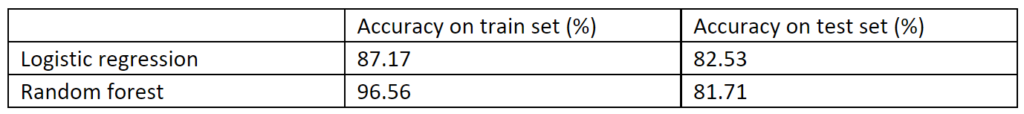
See that there is a small gap between train and test accuracy for the linear regression model. This is expected as linear regression is limited to linear divisions of the dataset. Moreover, it achieves a slightly better accuracy than the random forest in the test set. Therefore, the linear regression model generalizes better than the random forest and the random forest is overfitted. We may need to tune tree parameters to regularize them. But is this completely true? Accuracy is a tricky metric with unbalanced datasets. Moreover, we not only want to predict the right pattern, but we also want that when the right pattern is not the one predicted, at least, the chosen one should be as close as possible to the right one. In other words, exchanging patterns 2 and 8 (both Sunday patterns) may be acceptable but not exchanging pattern 2 for pattern 1.
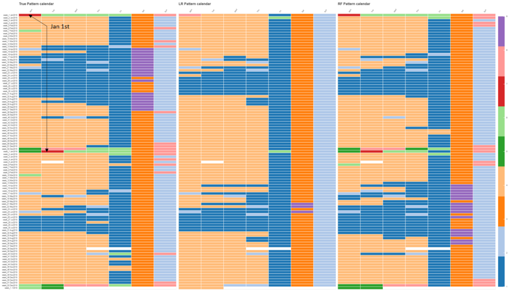
Comparing the predicted patterns calendars with the true one, we see that linear regression does an excellent job of distinguishing Sundays, Saturdays, Fridays, Mondays through Thursdays, and holidays, and it goes for the most common patterns for each of these types of days. On the other hand, it does a poor job on the weeks when Christmas and New Year fall. Conversely, the random forest does recognize days around Christmas as special ones and assigns them different holiday-related patterns with high accuracy. However, it also exchanges patterns 3 and 9 (Saturday patterns), 2 and 8 (Sunday patterns), which lowers the overall accuracy.
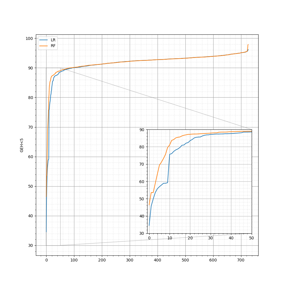
But as mentioned before, the objective is also to at least predict a good pattern when the best one is not chosen. If we compare the flow of the predicted pattern with the measured flow, we calculate the daily GEH<5, and we sort the values we obtain the next image. It shows how the random forest is superior for the worst 50 days.
I hope that this post has helped you to understand how supervised learning works and how it can be used. In this case we transformed a regression problem (predicting traffic value at various locations) into a classification problem (predicting the right pattern for the day). Once we defined the explanatory and target variables of the classification problem, we divided the dataset into 5-fold train-and-test sets, and we built two types of models for each fold and then analyzed the results. According to the results the random forest achieves a better performance, especially if we compare the worst 50 days for each type of model. Moreover, the random forest could choose “good enough” patterns aside from the best one, an ability that derives from the random forest’s non-linear division of the solution space and from the fact that the solution space had features that permitted this. We could call it “luck”, because we did not input any information about how close each pattern is to each other or how good each pattern is for each day. We only input the best pattern for each day assuming each pattern is equally different to each other. There are different ways of doing this, naturally, and in Aimsun we have chosen one. But that’s a topic for another day. 😊
From traffic forecasting perspective, we have seen how a next-day or several-days-ahead prediction problem can be formulated in terms of a classification problem. The fact of converting a “natural regression” problem into a classification problem is to alleviate the model from the burden of estimating a time-series for each sensor in the network. If we have a few loop detectors, it may not be important, but if we have thousands of them, we may end up increasing the size of the model proportionally to a function of the number of sensors, and usually this “function” is not linear. To put it in numbers, this methodology requires running a clustering algorithm and training a classification problem, that both can be run in seconds for large networks, instead of a large neural network that needs hours to be trained. Therefore, I encourage anybody trying to build a traffic forecasting system to, at least, use this methodology or a similar one as baseline to compare with other complex models.
