1. Introduction

Matrix Adjustment is a procedure for adjusting an a priori OD matrix, using traffic counts from detectors, detector stations, road sections or turns from nodes or super nodes. The solution algorithm is based on a bi-level model solved heuristically by a gradient-based algorithm which runs an assignment at each iteration. The algorithm calculates a sequence of OD matrices that consecutively reduce the least squares error between traffic counts coming from detectors and traffic flows obtained by a traffic assignment.

The algorithm used to solve the problem is heuristic in nature, of steepest descent type, and does not guarantee a global optimum for the formulated problem, so manual intervention is sometimes necessary to get a good result.

Aimsun Next provides several options to limit the adjustment process to prevent overfitting and to stay as close as to the original matrix, for example: matrix elasticity and trip length distribution elasticity can be set to globally limit any change from the original matrix; or, in some cases, a maximum deviation matrix can be provided to precisely set a limit of change for each individual OD pair; or the weight function can be used to assign different weights to the observed values (real data) used for the adjustment.

The use of the weight function is the least explored of these options. The weight function is the only option that directly influences the observed values, and furthermore, a known issue of the least squares error is that it favours high values. The weight function, if properly used, could reduce the imbalance between high and low counts and thus improve the overall adjustment result.

This technical note explores the impact of weight function on the matrix adjustment process.

2. Test model and data

The base demand for the OD adjustment is derived from the strategic model in Emme. The detector data used in this study are from two different sources: the motorway data collected from the motorway detectors which records individual vehicle counts at every 3 minutes. Most of the signalised intersection has intersection counts collected from SCATS historical database. SCATS data are stored at 1-5-minute intervals. The combined dataset has been updated at 15-minute intervals. These detector data are later combined with detector station data (a detector station on a multilane road section is a collection of detectors with a common direction of travel).

The model covers local roads to expressways and has a total of 1,236 detector stations, of which 203 are on motorways, and the rest on urban signalized intersections. The extent of the flow observed on different detectors ranges from 0 – 6,070 veh/hr.

3. Impact of weight function on matrix adjustment

3.1 Weight function

An adjustment weight function can be used as a form of the reliability of the real data (section/detector/turn counts) used for the adjustment process. By default, no weight function is applied. The following weight functions have been applied in this study:

Weight function 1 = (1/(observed Volume^0.2))*10
Weight function 2 = (1/(observed Volume^0.4))*50
Weight function 3 = (1/(observed Volume^0.6))*300

3.2 Impact of weight function on OD adjustment performance

To understand the effect of weight function on matrix adjustment, let’s take four different static OD adjustments: using no weight function, and using weight function 1, 2, and 3. The experiments had the following settings:

• Number of outer iterations = 20
• Number of gradient descent iterations = 3
• Number of inner iterations = 50
• Relative gap = 0.1%
• Assignment method = Conjugate Frank and Wolfe

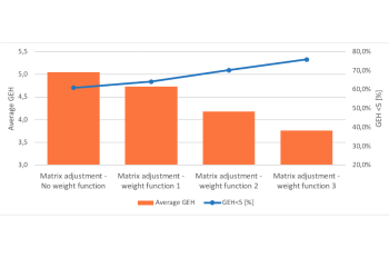
Table 1 presents the outcome of the matrix adjustment experiments. The performance of the adjustment is validated with the observed and simulated flow. The main criteria for validation are GEH<5%, average GEH level and regression R2.

Table 1 shows that even without using any weight function, the matrix adjustment does a good job. The GEH<5% for all data is around 61%, while for observed flow over 2000 it is 100%. A known issue of the matrix adjustment is that it favours high flow as the algorithm uses the least squares error between traffic counts coming from detectors and traffic flows obtained by a traffic assignment. Therefore, when we use a weight function that gives high weight to small counts, it is likely to improve the adjustment performance. Table 1 shows that using weight 3 improves the overall GEH<5% to 76%. The weight function has reduced the average GEH level.

Interestingly, the average GEH for observed flow over 2000 has increased with the increase of weight while the opposite is observed for flow below 2000. This behavior is caused by the nature of the weight function used in this study, which put greater weight on the small flows. Hence, the adjusted matrix showed better performance for local roads, i.e. roads with flow <2000 veh/hr.

Applying the weight function clearly improves the adjustment performance. However, the weight function is likely to cause more distortion in the original matrix compared to the adjustment with no weight function. For example, the following figure indicates the matrix distortion through the scatter plot of adjusted vs original demand. The regression R2 value for no weight and weight 3 are 0.8143 and 0.7138 respectively. Using weight 3 created more distortion to the original matrix to match the observed flow more closely.

The type of weight function affects the trip length distribution; for example, in this study, the weight function favours small flows which are likely to appear on local roads. Therefore, a high weight function will create more short length trips than no weight function (see the following figure).

From the above discussion, it is clear that weight function is a powerful tool for matrix adjustment. However, there is a danger of overfitting the model. A balance between the low and high flow areas of the network should be maintained by selecting an appropriate weight function.

Figure 4: Impact of weight function on matrix deformation and trip length distribution

3.3 Impact of gradient descent iteration on OD adjustment performance

In the bi-level optimization framework for matrix adjustment in Aimsun Next, the gradient descent method is executed without changing the path choice results obtained from the static assignment that was performed at the outer iteration. A higher gradient descent iteration should improve the matrix adjustment with the cost of higher run time. In the previous test, we used a gradient descent iteration of 3. In this section, we will observe the impact of the gradient descent iteration on matrix adjustment performance with no weight as the base case. Table 2 presents the effect of gradient descent iteration on matrix adjustment performance. No weight function has been used.

A close observation of the changes in average GEH or GEH<5 % shows a rapid change in matrix adjustment performance between iteration number 1 and 3. The changes in adjustment performance from gradient descent iteration 3 to 9 are almost linear. Therefore, in the rest of the analysis, a gradient descent iteration = 3 has been used.

The improvement in matrix adjustment comes with higher deformation of the original demand and trip length distribution. In Figure 6, a comparison of matrix deformation and trip length distribution is shown between gradient descent iteration 1 and 7. The regression R2 has reduced to 0.77 with 7 gradient descent iteration compared to an R2 value of 0.88 with only 1 gradient descent iteration. Similarly, a higher number of short trips is observed with the increase of gradient descent iteration.

4. Impact of weight function on matrix distortion

So far, the analysis was performed on real data collected from different sources. The base demand comes from a strategic model. As the data used for adjustment comes from different sources, it is difficult to know which is more reliable. By imposing different weight or controlling other parameters the adjustment process produces an output which has been distorted from the input(base) matrix to fit the counts. However, we have no idea about how close the adjustment result is to the true matrix. True matrix is a hypothetical matrix that would (if available) produce the same detector counts.

In this section, we performed a hypothetical test to observe whether the weight function helps to produce a demand matrix that is close to the true demand. We have observed that weight function provides better performance for matrix adjustment. However, the better performance comes with the cost of higher deformation of the input matrix and higher changes in trip length distribution. It would be interesting to know whether these changes have produced a matrix that is closer to the true matrix. If the result is closer to the true matrix, then the higher deformations to the input matrix should be acceptable.

4.1 Creation of true and synthetic demand and RDS from true demand

We have taken the adjusted demand from section 3.2 with weight function 3 (as it produced the best adjustment outputs). We have taken this demand as the ‘true demand’. The equilibrium flow generated from this true demand at the detector stations is named as the true RDS. This true RDS is a perfect RDS that is free from any observation error, and all the detector flow are consistent with the upstream, downstream flows as well as among all other approaches of an intersection.

The true demand has been distorted by adding a white noise and named as ‘synthetic demand’ that will be used for matrix adjustment. The white noise is produced from a normal distribution with mean = 0 and standard deviation = 0.5, seed = 1. The synthetic demand is created following this formula:

Where i and j denote origin and destination respectively.

In the real world, we don’t have access to this ‘true demand’. We will only have access to the ‘synthetic demand’. Hence, this test will provide some valuable insight into how close the adjustment can bring the matrix close to the original/true demand.

4.2 OD adjustment result with synthetic demand and true RDS

Table 3 presents the result from the adjustment with synthetic demand and true RDS. As we had observed before the weight function did a good job. Even without using the weight function the result is good. The reason is most likely due to the quality of RDS. As the RDS is free from inconsistency in flow, the adjustment process had less trouble in finding global minima.

As we now have access to both the true and synthetic matrix, we can compare the quality of the adjusted matrix. Table 4 presents the regression R2 values between the adjusted and the true demand. It also shows the regression R2 values between the adjusted and the synthetic demand.

The weight function has created more deformation to the synthetic matrix that has been used for the adjustment (the regression R2 between synthetic and adjusted demand is the lowest for weight function 3 and highest for no weight case). Interestingly, the opposite is observed for the true demand. This high deformation has taken the matrix closer to the true matrix. The regression R2 between the adjusted and the true demand is the highest for weight function 3 and lowest for no weight case. Clearly, the weight function has deformed the matrix in the right direction to create an adjusted demand that closely represents the true demand.

5. Summary

• Use of adjustment weight function can significantly improve the matrix adjustment performance.
• In most of the project the aim is to attain a high GEH <5 percentage. The normal adjustment process maximises the R2 value, however it has no control on the GEH.
• This study finds a close relation between the weight function and GEH. Increasing the weight function has helped to reduce the average GEH level and increases the GEH <5 percentage.
• Weight function creates higher deformation to the base matrix compared to adjustment with no weight function — also, the trip length distribution changes to some extent.
• A high gradient descendent iteration helps to improve the adjustment performance.
• A gradient descent iteration ≥ 3 is recommended.
• RDS quality has a big impact on the adjustment performance.
• If we can ensure the RDS consistency, a weight function can lead the adjusted matrix close to the true matrix from where the RDS would have been derived.